End Semester Update on GPS

16 Apr 2018

As the semester dwindles down, I’d first like to say I’m proud of everyone who has put in all the hard work this past year.

Without the collective effort of the team, there’s no way we could have ever gotten to this point. So, congrats guys, we’ve made it this far! Let’s keep it up for the long haul.

That being said, with competition looming overhead in about 6 weeks time, we still have quite a bit of work left to do. As of today, we’ve only just begun our final transition from simulation testing to fine-tuning in the real world. Here’s a quick snapshot of what we’ve been working on.

GPS Waypoint Following:

After covering both obstacle avoidance and lane detection in previous blog posts, waypoint following is the last big criteria we’re aiming to hit. In the past month alone, we have gone from virtually nonexistent waypoint navigation to pretty damn good results. In a nutshell, here’s our basic outline.

First Step: Raw Data

Using last year’s VectorNav VN200 INS/GPS sensor, we are actively polling for longitude and latitude coordinates. Previous tests have shown that our sensor yields an average error of approximately 0.4195 meters in any given direction. Not quite the centimeter level resolution we were looking for, but it’ll do.

Although this resolution isn’t good enough for decent odometry data alone, it’s definitely well built for simple point to point navigation. Using the haversine formula, we can approximate the distance and bearing from RAScal’s current position to a specified waypoint (they’ll be giving us these at competition).

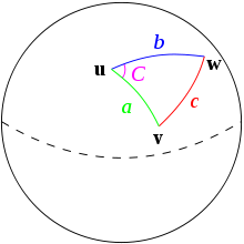
Figure 1. Geometric Representation of Bearing and Distance

Up Next: PID Controllers

For those of you who have been following along closely, the same VN200 sensor is also being polled for yaw heading directions. Given the direction of where we are heading (local yaw), as well as the bearing of where we should be heading (compass yaw), we can calculate an approximate error from a setpoint. For those familiar with PID controllers, this is a perfect time to implement said control loop.

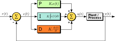
Figure 2. Block Diagram of Closed-Loop PID Control

Buckle up, boys and girls, we’re heading into the magical world of mathematics. In a nutshell, all we are trying to do is to bring our local yaw heading to line up with the direction of the compass bearing as fast as possible, without any overshoot, delays or any of the fun bits and pieces involved with complex motion.

The simplest implementation is a P controller. Take your setpoint, which in our case is the compass bearing, subtract the yaw heading, and multiply that error difference by a constant, denoted P-gain.

If we scale this output proportionally to the vehicle dynamics of our robot, we can drive motors faster or slower depending on how off we are from the setpoint.

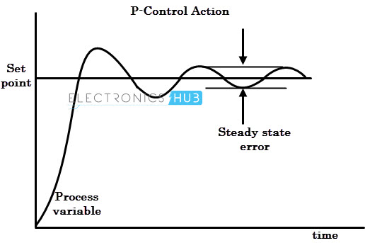
Figure 3. P Controller in Action

Now you may be wondering, what happens when we begin to approach the setpoint? The difference between our local yaw heading and the setpoint will begin to diminish rapidly. Eventually, we would incur what is known as Steady state error. The answer to this, is the integral component of our PID controller.

If you have taken virtually any calculus class, you’ll know that integrals are these absolutely wonderful things with flowers and butterflies blooming all around. Over time, as we add up, or take the summation of our error values, we can eventually blow up this integral term, enough that even small residual error is noticeable. It only takes a few iterations to get the ball rolling.

In any other case, we’d be done right about now. PI controllers work well, and there isn’t much to say otherwise. However, we ultimately decided, oh why not, let’s do a full PID controller instead. This is precisely where the derivative component comes into play.

The derivative component works well in our case because we also want to avoid jerky motion. By measuring in this case, not the overall summation of error, but rather the changes in error over time, we can get a good estimate of how we are turning to reach our setpoint.

If we turn too quickly, our derivative term grows (in the negative direction), thereby eventually dampening RAScal’s turning motion. This works especially well when we want to reach our setpoint without major overshoot while still turning at a fairly rapid pace.

Final Steps: Motor Commands

Now that we have all these terms, what do we do now? Thinking in terms of whole process, our end goal is to simply turn such that our local yaw heading matches with the calculated compass bearing. In our case, the output from this PID controller then becomes the velocity commands we send to each individual motor. The relative speed at which we turn each motor, is governed by the output from our controller. Poll the raw data again, and we start all over again.

Looking Ahead:

One thing you’ll notice in the equations above is that they all have a K-constant involved. These are called PID gains, one gain for each term. Tuning these gains is a fairly involved process. Good ol’ Ziegler-Nichols can help us out with that.

However, arguably more of a priority right now, is filtering odometry data. Once we get our encoders up and running, we’re going to need GPS to work in tandem with our encoders. If we can filter our GPS data with an Extended Kalman Filter or the like, as past years’ teams have done it, our odometry data will be golden.

On top of all this, Vivek Malneedi has been working on porting, I believe it was ORB-SLAM 2, over from C++ to python code. Luckily for us, visual odometry is a thing so once all these odometry sources fall into place, we’re even better off than just a couple sources.

As always, I welcome you to come check out IGVC meetings weekly, Fridays at 4PM, EER 0.822. Thanks for reading! Slack Channel: #igvc

Author: Ricky Chen

---